Credit Risk Analytics
What really drives loan affordability risk?
Our team built a credit risk business case around Nationwide and analysed 44,986 public loan records in SPSS, auditing the data before using correlation and multiple regression to test which factors drove the loan to income ratio.
Loan amount drove affordability pressure (β = .767). Credit score and interest rate were not significant.
Explore the evidence ↓01 · Decision
Our team defined the decision before selecting a method.
Which borrower and loan characteristics drive affordability pressure, measured as the loan to income ratio, and do commonly assumed signals such as credit score and interest rate still matter once the other factors are considered?
The most useful result was what did not predict affordability.
You might expect credit score and interest rate to lead any affordability model. Once loan size and income were included, neither was statistically significant: loan amount (β = .767) and income (β = −.488) carried the model. A credit team would want to challenge and investigate a result like that, not ignore it.
The judgement in the work
We flagged implausible records before modelling, such as 100 years of work experience recorded for a 35 year old, and checked the diagnostics afterwards. Heteroscedasticity in the residuals meant individual coefficients needed careful reading, which is why I would use robust standard errors in the next iteration.
02 · Approach
Our team organised the analysis in the following sequence.
- 01
Our team framed a credit risk problem statement and objectives for a Nationwide case study, using a public Kaggle loan dataset.
- 02
We profiled the 44,986 records with descriptive statistics and flagged implausible values, such as employment experience of up to 100 years for borrowers aged 35, before modelling.
- 03
We used Pearson correlation to screen the relationships between the loan to income ratio and the candidate predictors.
- 04
We dummy coded the categorical variables and fitted a 12 predictor multiple linear regression in SPSS.
- 05
We checked the assumptions with PP and residual plots, residual statistics and variance inflation factors, then translated the results into lending recommendations.
03 · Evidence
The results support the following interpretation.
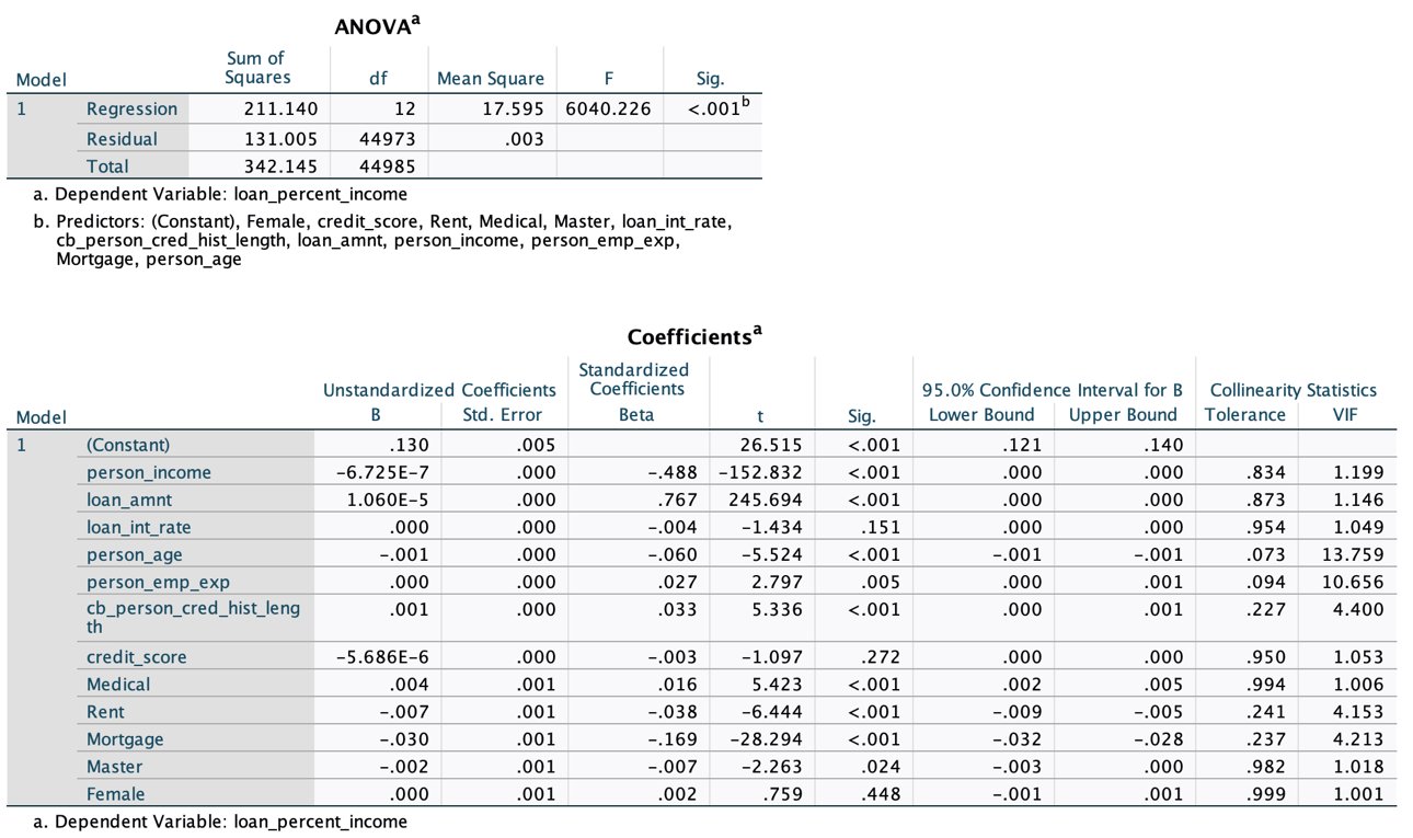
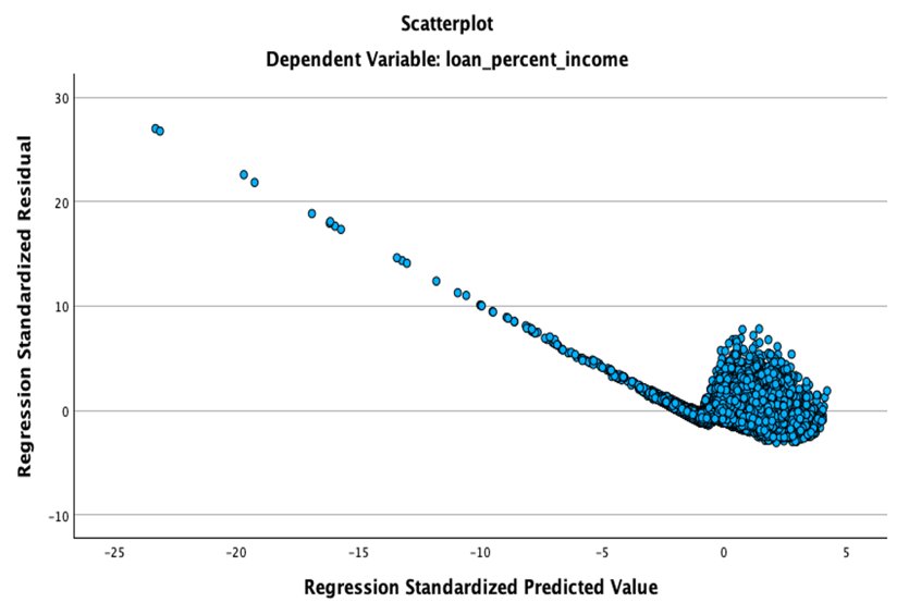
The model explained 61.7% of the variance in the loan to income ratio (R² = .617; F(12, 44973) = 6040.23, p < .001). Loan amount was the strongest predictor (β = .767) and income the strongest protective factor (β = −.488). Interest rate (p = .151) and credit score (p = .272) were not significant once the other factors were included. The diagnostics showed nonnormal, heteroscedastic residuals, standardised residuals of up to 27 and high VIFs for age (13.8) and employment experience (10.7), so individual coefficients need careful reading.
ANOVA and coefficients
The full regression output for the loan to income ratio, including standardised coefficients, confidence intervals and the collinearity statistics behind the VIF warning.
Source: SPSS output screenshot from the submitted team report.
Residuals against predicted values
The funnel shape and long diagonal tail are why the report flags heteroscedasticity and extreme outliers, and why robust standard errors are the next step.
Source: SPSS diagnostic plot from the submitted team report.
04 · Decision implications
Our team translated the analysis into practical next steps.
- Size loans relative to income first: exposure and repayment capacity explained affordability pressure far better than credit profile alone.
- Look beyond income thresholds, because some higher income borrowers still carried high loan to income ratios.
- Clean implausible records before modelling, and report diagnostics next to coefficients so decision makers know how much weight each result can carry.
05 · Limits
The evidence has defined limits.
This was an assessed case study on a public dataset, not Nationwide’s own data or a production credit model. The data is cross sectional, so the results show association rather than causation, and they lack expenditure and housing cost data. The heteroscedasticity and outliers mean robust standard errors are needed before relying on individual coefficients.
06 · Next iteration
Our team would strengthen the next iteration.
Use heteroscedasticity robust (HC3) standard errors, as I later did in my dissertation, remove one of the collinear age or experience variables, add t tests and ANOVA across borrower groups, and compare against a nonlinear model such as gradient boosting.
07 · Attribution
I distinguish my contribution from the complete project output.
This was a four person team project with shared responsibilities, so the data audit, modelling and recommendations are described as our team’s work.
Toolkit